In November 2014 I found myself on Estes Rockets’ website looking at their Black Friday sale. The only experience I had with model rockets was from a weekend at summer camp over a decade prior. But with the prices of some low power kits at $4 I figured building them could be a fun rainy weekend activity. A week and $30 later a box full of six rockets came in the mail and then proceeded to collect dust in my closet until one uneventful weekend in May when I decided to at least open the package. I had foolishly underestimated the amount of time it takes to assemble even a simple low power rocket (my vision of building all of them in a single evening was not realistic), but the next weekend I headed down to the local park with the assembled rockets, a pack of motors, and a launch pad I made out of PVC pipe. It was fun, I thought, but launching small rockets 500ft up doesn’t hold one’s attention for very long. That’s when I discovered the world of high power rocketry and an active community in my city. After attending a few meetings with the local NAR club, I loaded up my car and headed out to the last high power launch of the season with the intention of getting a level 1 high power rocketry certification. Being my first high power launch, I was not expecting just how high and far downrange these rockets can go. Despite seeing my rocket come down I misjudged how far out it was and spent the remainder of the afternoon wandering around a field full of mud, thick brush, and mosquitoes that I would not want to spend ten minutes walking through. Long story short, I did eventually recover the rocket, but I had plenty of time to think about how I was never again launching a rocket without a tracking system installed.
The original vision for my tracking system, Osprey, was an Arduino Pro Mini connected to a GPS receiver and radio transmitter. A radio receiver on my laptop would read the GPS coordinates and plot the rocket’s current location on a map. Simple enough, right? Well, as is my style, things got a little out of hand from there. I figured that I might as well add an altimeter since it would be nice to know how high my rockets were actually going. For a few dollars more I learned that I could get a full IMU. That is, a barometer, three-axis accelerometer, gyroscope, and thermometer. I then decided that it would be nice to log all of this data for post-flight analysis. I then added a micro SD card to log all of the data to. At this point I was well beyond the capabilities of an Arduino so a more powerful ARM board was needed. On the software side, I figured that if I’m collecting all of this data, I might as well graph it in real time so a GUI was built for that. Next I decided that I wanted my next rocket to be dual deploy so I needed to build an igniter circuit and the associated software to detect apogee and fire the deployment charges at the right time. This also meant that rather than simply sending data from the rocket to my laptop that I would need to send commands to the rocket so two directional communication support was added. From my testing in low power rockets of what I had so far, I realized that it was impractical to carry my laptop around a launch site collecting data. Thus, an Android app was created to replace the desktop application for receiving data. During the build of my new rocket, I became concerned about losing it due to some software bug so I embarked on writing a way to simulate flights and a test suite for the embedded code. And finally, I decided that it would be interesting and fun to write a “small” launch report generation script that would take a log file from a flight and generate a static HTML page with relevant stats, graphs, and a 3D flight path and rocket orientation playback.
So yeah, you could say what I ended up with was a bit outside of the original scope.
Now, eight months later, I ended up with a tracking, telemetry, and dual deployment system with three different clients, test suite, and automatic report generation. Build and usage documentation are location in Osprey’s repo on GitHub, so here I’d like to go into detail about some of the more interesting components of the project.
Sensor Noise Filtering
One of the first issues run into when working with rapidly and continuously changing sensors like accelerometers or gyroscopes is noise. There are many ways to handle this, but the go-to choice for embedded systems is usually a Kalman filter. In a highly simplified nutshell, a Kalman filter essentially makes an educated guess on what the next data point will be based on the current data point. Then depending on how much the next data point differs from the current, it will weight the actual value verses the predicted value accordingly. What we’re left with is a relatively simple and lightweight method for extracting meaningful trends from noisy data in real time.
This is simple enough in theory, but the implementation gets much more hairy. There are both simple one-dimensional Kalman filters and more complicated multidimensional filters. For my purposes the one-dimensional variant was sufficient. Beyond being relatively easy to understand, the other advantage is that its implementation is simple, uses little memory, and is not computationally intensive; all very desirable traits for an embedded system. Below is the implementation pulled from the Sensor class used in Osprey.
1
2
3
4
5
6
7
8
9
10
11
12
13
14
15
16
17
18
19
20
21
22
23
24
25
26
27
28
29
30
31
32
33
34
typedef struct {
  float processNoise;     // process noise covariance
  float measurementNoise; // measurement noise covariance
  float value;            // value
  float error;            // estimation error covariance
  float gain;             // kalman gain
} kalman_t;

Sensor::Sensor(float processNoise, float measurementNoise, float error) {
  this->processNoise = processNoise;
  this->measurementNoise = measurementNoise;
  this->error = error;
}

kalman_t Sensor::kalmanInit(float initialValue) {
  kalman_t kalman;

  kalman.processNoise = processNoise;
  kalman.measurementNoise = measurementNoise;
  kalman.error = error;
  kalman.value = initialValue;

  return kalman;
}

void Sensor::kalmanUpdate(kalman_t* state, float measurement) {
  // Prediction update
  state->error = state->error + state->processNoise;

  // Measurement update
  state->gain = state->error / (state->error + state->measurementNoise);
  state->value = state->value + state->gain * (measurement - state->value);
  state->error = (1 - state->gain) * state->error;
}
As you can see, it’s actually a short amount of code. The magic happens in the kalmanUpdate method. The value is a function of the previous value, the gain, and the current value. The gain is a function of the error and measurement noise. That’s easy enough, but you’re probably wondering what the initial value, process noise, and measurement noise, constants are. Each system is different so they will vary wildly, not just between projects, but between individual sensors. The short answer is that picking these values is more of an art than a science. The approach taken with Osprey was to adjust the values and graph the raw versus filtered data until an acceptable tradeoff between quickly updating values and noise reduction was found. For reference, these are the values Osprey uses for each of its sensors:
1
2
3
#define KALMAN_PROCESS_NOISE 0.01
#define KALMAN_MEASUREMENT_NOISE 0.25
#define KALMAN_ERROR 1
If you’re interested in learning more about Kalman filters, there is a mountain of information available on the web by people much more knowledgeable on the topic than myself. For instance, this is a particularly informative introduction to the topic.
GPS Filtering
Filtering the GPS coordinates required a different approach than a Kalman filter. Consider the following latitude and longitude data:
1
2
3
4
5
6
7
47.817749, -119.656333
47.817748, -119.656332
47.817747, -119.656331
47.000000, -119.000000
47.817746, -119.656330
47.817745, -119.656329
47.817744, -119.656329
This is manufactured data based off of a flight log and from my memory of the type of data received from the GPS receiver.
The signal to noise ratio here is actually fairly high. It’s the occasional data point that comes in corrupt or otherwise incorrect. Practically speaking, this doesn’t cause much of an issue; the location of the rocket is still known. The problem arises when putting the flight path on a map. Even small changes in coordinates mean significant changes in location on the Earth’s surface. Having anything but perfectly clean data is going to result in massive spikes in the flight path on the map. And if these incorrect coordinates occur, say, even 1 out of 30 data points, over the course of an entire flight this leads to a large number of spikes on the flight path which is distracting at best.
Filtering the incoming data with a Kalman filter does not solve the problem since any far out of range value would still cause somewhat of a spike in the filtered data. Moreover, since the rocket can conceivably be located anywhere on Earth, a band filter could not be used either without waiting to establish some history of data points.
The approach taken instead was to ignore values that were outside of a given range. The number of continuous values that were outside of the range was tracked and if a certain number of out of range data points were encountered, then begin treating those as the valid points and only accept new data points within the given range of them. It’s something like a dynamic band filter; I’m not sure if there is a formal name for this type of filter.
Here’s the implementation:
1
2
3
4
5
6
7
8
9
10
11
12
13
14
15
16
17
18
19
20
21
22
23
24
25
26
27
28
#define OUT_OF_RANGE_DELTA 0.001
#define OUT_OF_RANGE_LIMIT 5

int GPS::validCoordinate(float previous, float next, int *outOfRange) {
  // If we keep reading seemingly invali coordinates over and over, they're probably valid
  if(*outOfRange > OUT_OF_RANGE_LIMIT) {
    *outOfRange = 0;
    return 1;
  }

  // Ignore ~0.00 coordinates (obviously doesn't work if within 1 degree of the equator or meridian, but good enough for now)
  if(next < 1 && next > -1) {
    return 0;
  }

  // Ignore anything greater than the out of range delta from the previous coordinate as there's
  // no way to move that fast except in the case of initially acquiring a location when the
  // previous coordinate will be 0
  if(previous != 0 && abs(next - previous) > OUT_OF_RANGE_DELTA) {
    (*outOfRange)++;
    return 0;
  }

  // Reset the out of range counter if valid
  *outOfRange = 0;

  return 1;
}
Apogee Detection
Detecting when the rocket is at apogee is a seemingly simple problem to solve. However, it’s complicated by two difficult issues:
- Detecting apogee too early means deploying a parachute at high speed, possible ripping the parachute off and damaging or resulting in the loss of the rocket.
- Detecting apogee too late also means deploying a parachute at high speed or, even worse, not detecting it at all leading to the rocket entering lawn dart mode.
For these reasons, it is imperative to have meaningful data to rely upon for apogee detection calculations. With the filters above to ensure that is the case, we’re free to look at how to detect apogee from our data.
Apogee detection with the barometer
Logically, it would seem that apogee detection is easy given altitude data: whenever the altitude transitions from increasing to decreasing, that must be apogee. There are two problems with this:
- The name of the game here is accuracy. If we detect apogee at the wrong time or not at all it could result in the loss of the rocket. Thus, it would be careless to detect apogee by looking for a single altitude data point that is less than the previous point. In order to provide the level of confidence needed we would need to keep a history of altitude data points and say some X number of decreasing points probably means apogee. This is both memory and computationally intensive, but the real issue is that this cannot be done in real time. Apogee detection would always take place after actual apogee. Sure, it may be “close enough,” but we can do better.
- A funny thing happens when an object transitions to/from supersonic speeds. As the shockwave passes over the barometer it will sense the increased pressure which will lead to a suddenly lower altitude reading. This is yet another reason why the barometer data is filtered with a Kalman filter, but a dramatically lower reading could be enough to cause at least one data point that shows decreasing altitude triggering the scenario outlined in the point above.
That said, it is correct to say that the altitude data from the barometer provides useful information when used in conjunction with other sensors. We will revisit this shortly.
Apogee detection with the accelerometer
Another option to detect apogee is through the use of the accelerometer. We know that at apogee the rocket will be weightless so a reading of 0g means that the rocket is at apogee.
There are two important items that make using the acceleration a viable method of apogee detection:
- The accelerometer I’m using is a three-axis accelerometer. Using a single axis works only if the rocket will remain perfectly straight during flight, which is rarely the case. Having all three axes allows us to not have to worry about rocket’s orientation in space. In fact, with this data, the total acceleration is determined as follows:
atotal = (ax2 + ay2 + az2)1/2. Then, regardless of orientation, it’s possible to check if the rocket is accelerating, decelerating, or weightless. - The accelerometer I used has a range of -2g to 2g. This has the downside of not being able to capture the true force at liftoff due to it being out of range, but for all other phases of flight, the small range means lower sensitivity which leads to more easily filterable and meaningful data.
Vertical velocity calculations
It’s worth mentioning that given the time and that the initial velocity of the rocket is 0, we could find the rocket’s vertical velocity with the equation v = v0 + 1/2at2 and check if the velocity is 0 for apogee detection. In fact, this is how some other flight computers detect apogee. However, in my experience, this works great in theory, but in practice error in the acceleration measurement quickly builds up to the point that the derived velocity is essentially useless. Even with filtering of the accelerometer data, my experiments with this method always resulted in velocities that were not remotely accurate. It may be that my Kalman implementation could be vastly improved, but regardless, I was not finding a high enough level of reliability to suit my purposes. Thus, I decided to stick with the acceleration itself as my apogee detection heuristic.
Accelerometer & Barometer
With the total acceleration known and that data being filtered to remove noise, it’s possible to get a rough idea of when apogee is occurring, but to be as accurate possible, we bring the barometer and its altitude measurements back into the mix. From here, it’s a matter of developing logic for determining when the rocket is at apogee. Osprey’s implementation utilizes four primary methods of doing this:
- With the acceleration close to 0g (<0.15g) begin watching the altitude from the barometer. When it decreases, we’re at apogee. Also start a countdown so that if a decreasing altitude is never detected, an apogee event will still occur.
- With the acceleration somewhat close to 0g, (<0.3g), start a safety countdown so that if the lower acceleration threshold is never hit, an apogee event will still occur.
- As a final fail safe: If the acceleration is greater than 1g again and we’re looking for apogee (the rocket is in the coast phase of flight), fire the apogee event because we failed to detect apogee entirely.
- A manual override command may also be sent from the ground to immediately cause an apogee event.
The full apogee detection function is as follows:
1
2
3
4
5
6
7
8
9
10
11
12
13
14
15
16
17
18
19
20
21
22
23
24
25
26
27
28
29
30
31
32
33
34
35
36
37
38
39
40
41
void Event::phaseCoast(float acceleration, float altitude) {
  // If apogee is pending, as soon as the altitude decreases, fire it
  if(pendingApogee) {
    if(previousAltitude - altitude > APOGEE_ALTITUDE_DELTA) {
      atApogee(APOGEE_CAUSE_ALTITUDE);
    }
  }

  // If the apogee countdown is finished, fire it
  int apogeeCountdownCheck = checkApogeeCountdowns();
  if(apogeeCountdownCheck > 0) {
    atApogee(apogeeCountdownCheck);
    return;
  }

  // Anything less than the ideal acceleration means we're basically at apogee, but should start paying attention to altitude to get as close as possible
  if(acceleration < APOGEE_IDEAL) {
    pendingApogee = 1;

    // Only start the countdown if it's not already started
    if(apogeeCountdownStart == 0) apogeeCountdownStart = Osprey::clock.getSeconds();

    return;
  }

  // Anything less than okay acceleration is /probably/ apogee, but wait to see if we
  // can get closer and if not, the timer will expire causing an apogee event
  if(acceleration < APOGEE_OKAY) {
    // Only start the countdown if it's not already started
    if(safetyApogeeCountdownStart == 0) safetyApogeeCountdownStart = Osprey::clock.getSeconds();

    return;
  }

  // If the acceleration is back to 1 then we're falling but without a drogue chute (uh oh)
  if(acceleration > 1) {
    atApogee(APOGEE_CAUSE_FREE_FALL);
    phase = DROGUE;
    return;
  }
}
The constants used here were determined experimentally. That is, from looking at previous flight logs from mid-power flights and matching up acceleration values with altitude values. In high power flights since then, apogee detection has proven reliable; never has it not fired when it should have. There remains room for optimization to minimize the delta between calculated apogee and actual apogee, but the overall methods of apogee detection have proven themselves viable.
Testing
Testing software is, of course, always a good practice to follow. In this case, however, after sinking $500+ into a rocket that could easily be lost due to a software bug, testing was paramount.
The problem was that, unlike other software I had worked with, I had never tested an embedded system. The code I was writing was compiled to ARM, but I was writing it on an x86 machine. To add to that, I was using libraries unique to the processor on the microcontroller. Sure, I could probably find a way to test directly on the board, but it would be slow, inefficient, and problematic to run a test suite with test fixtures directly on the board itself. Rather, I thought, the one of the reasons for standard C and C++ is so that it can compiled to numerous architectures. So instead of testing directly on the board, I would provide stubs for the sensors and then compile the code to x86 so I could run it directly on my development system.
As a pleasant surprise, this proved an easier task than I had anticipated (that rarely happens!). One challenge was providing stubs for the Arduino libraries such as the analogRead() function, but this essentially boiled down to simply:
1
2
3
4
5
6
7
8
float analogRead(int pin) {
  return 0;
}

void delay(int ms) {}
void pinMode(int pin, int mode) {}
void digitalWrite(int pin, int mode) {}
void pinPeripheral(int pin, int mode) {}
Plus some others which are omitted here since they are mostly empty functions.
The ARM Cortex M0 processor has six “SERCOM” ports which are basically multiplexers for SPI, I2C, and UART ports. They allow the programmer to chose any combination of the three for use in the six ports that the processor supports. In my case, I was using two of them for serial communication with the GPS and radio. Stubbing the Uart class out meant that I could send and receive data with the now simulated board. My stub was:
1
2
3
4
5
6
7
8
9
10
11
12
13
14
15
16
17
18
19
20
21
22
23
24
25
26
27
28
29
30
31
32
33
34
35
36
37
38
39
40
41
42
43
44
45
46
47
48
49
50
51
52
53
54
55
#include "uart.h"

SERCOM sercom1;
Uart Serial1;

Uart::Uart() {
  bufferReadPosition = 0;
  bufferWritePosition = 0;
  echo = 0;
}

Uart::Uart(SERCOM *sercom, int a, int b, int c, int d) {}
void Uart::begin(int pin) {}

void Uart::write(char c) {
  if(echo == 1) {
    putchar(c);
  }
}

int Uart::available() {
  return (bufferWritePosition - bufferReadPosition > 0);
}

char Uart::read() {
  char c = buffer[bufferReadPosition];
  bufferReadPosition++;

  if(bufferReadPosition >= BUFFER) {
    bufferReadPosition = 0;
  }

  return c;
}

void Uart::insert(const char *buffer) {
  for(int i=0; buffer[i] != '\0'; i++) {
    this->buffer[bufferWritePosition] = buffer[i];
    bufferWritePosition++;

    if(bufferWritePosition >= BUFFER) {
      bufferWritePosition = 0;
    }
  }
}

void Uart::IrqHandler() {}

void Uart::enableEcho() {
  echo = 1;
}

void Uart::disableEcho() {
  echo = 0;
}
Essentially all it does is implement its own circular buffer. The test driver puts data into the buffer and the radio class in Osprey can come along and read it as normal without ever knowing it is running in a test environment instead of on the actual microcontroller.
For stubbing out the sensors, my own Stub class would read sample data from a JSON file and then put it into a map that could be read by child classes of the Stub class unique to each sensor. The Stub class handled the parsing of the JSON file as such:
1
2
3
4
5
6
7
8
9
10
11
12
13
14
15
16
17
18
19
20
21
22
23
24
25
26
27
28
29
30
31
32
33
34
35
36
37
38
39
40
41
42
43
44
45
46
47
48
49
50
51
52
53
54
55
56
57
58
59
60
61
62
63
64
65
66
67
68
69
70
71
72
73
74
#include "stub.h"

using string = std::string;
using map = std::map<std::string, stub_t>;

FILE* Stub::file;
map Stub::current;

field_t Stub::fields[] = {
  {"delta", FIELD_INT},
  {"expected_apogee_cause", FIELD_INT},
  {"expected_phase", FIELD_INT},
  {"latitude", FIELD_FLOAT},
  {"longitude", FIELD_FLOAT},
  {"pressure_altitude", FIELD_FLOAT},
  {"raw_acceleration", FIELD_FLOAT},
};

int Stub::open(const char *input) {
  file = fopen(input, "r");
  return (file != NULL);
}

int Stub::read() {
  if(file == NULL) return 0;

  char buffer[BUFFER];

  if(fgets(buffer, BUFFER, file) == NULL) {
    return 0;
  }

  // Go around again if a blank line or comment
  if(*buffer == '\n' || *buffer == '/') return read();

  json current = json::parse(buffer);
  updateMap(current);
  SERCOM1_Handler();

  return 1;
}

void Stub::updateMap(json current) {
  // Update each of the defined fields
  for(unsigned int i=0; i<sizeof(fields)/sizeof(fields[0]); i++) {
    string field = fields[i].field;

    // Only update the field if it exists in the json object
    if(current.find(field) != current.end()) {
      stub_t data;

      if(fields[i].type == FIELD_FLOAT) {
        data.floatVal = current[field];
      } else {
        data.intVal = current[field];
      }

      this->current[field] = data;
    }
  }
}

void Stub::close() {
  fclose(file);
  file = NULL;
}

stub_t Stub::getField(string field) {
  return current[field];
}

void Stub::setField(std::string field, stub_t data) {
  current[field] = data;
}
Where a union helped keep multiple data types inside of a single map to reduce overhead and a field struct tracked what data type each field was:
1
2
3
4
5
6
7
8
9
union stub_t {
  int intVal;
  float floatVal;
};

struct field_t {
  std::string field;
  int type;
};
Lastly, I created a stub class for each sensor that inherited from the parent Stub class with the same methods as the class that was responsible for actually reading data from the physical sensor. Here’s the stub for the barometer:
1
2
3
4
5
6
7
8
9
10
11
12
13
14
15
16
17
18
19
20
21
22
#include "Adafruit_BMP085_Unified/Adafruit_BMP085_U.h"

Adafruit_BMP085_Unified::Adafruit_BMP085_Unified(int32_t sensorID) {}

bool Adafruit_BMP085_Unified::begin() {
  return true;
}

void Adafruit_BMP085_Unified::getTemperature(float *temp) {
  *temp = getField("temp").floatVal;
}

float Adafruit_BMP085_Unified::pressureToAltitude(float seaLevel, float atmospheric, float temp) {
  return getField("pressure_altitude").floatVal;
}

bool Adafruit_BMP085_Unified::getEvent(sensors_event_t *event) {
  event->pressure = getField("pressure_altitude").floatVal;
  return true;
}

void Adafruit_BMP085_Unified::getSensor(sensor_t*) {}
As you can see, our work is cut out for us. All that’s necessary to do is read the current value from the map holding the sample data and return it. At this point, the implementation of apogee detection, command handling, and any other behavior on the board can be simulated.
For instance, we can define expected behavior in a test fixture and ensure that the flight would behave as expected given those inputs:
1
2
3
4
5
6
7
8
9
10
11
12
13
14
15
16
17
18
19
20
21
22
23
24
25
26
27
28
29
30
31
32
// Pad
{"raw_acceleration": 1.0, "pressure_altitude": 100, "expected_phase": 0, "delta": 0, "expected_apogee_cause": 1}

// Boost
{"raw_acceleration": 2.5, "pressure_altitude": 1000, "expected_phase": 1, "delta": 1}
{"raw_acceleration": 2.0, "pressure_altitude": 1000, "expected_phase": 1, "delta": 2}
{"raw_acceleration": 1.5, "pressure_altitude": 1000, "expected_phase": 1, "delta": 3}
{"raw_acceleration": 1.0, "pressure_altitude": 1000, "expected_phase": 1, "delta": 4}
{"raw_acceleration": 0.75, "pressure_altitude": 1000, "expected_phase": 1, "delta": 5}

// Coast
{"raw_acceleration": 0.74, "pressure_altitude": 2000, "expected_phase": 2, "delta": 6}
{"raw_acceleration": 0.5, "pressure_altitude": 2025, "expected_phase": 2, "delta": 7}
{"raw_acceleration": 0.4, "pressure_altitude": 2050, "expected_phase": 2, "delta": 8}

// Apogee (okay -- starts safety countdown)
{"raw_acceleration": 0.25, "pressure_altitude": 2100, "expected_phase": 2, "delta": 9}

// Apogee (ideal)
{"raw_acceleration": 0.1, "pressure_altitude": 2200, "expected_phase": 2, "delta": 10}

// Altitude less than previous step... should fire drogue
{"raw_acceleration": 0.1, "pressure_altitude": 2198, "expected_phase": 3, "delta": 11}

// Drogue
{"raw_acceleration": 1.0, "pressure_altitude": 1000, "expected_phase": 3, "delta": 12}

// Main
{"raw_acceleration": 1.0, "pressure_altitude": 250, "expected_phase": 4, "delta": 13}

// Landed
{"raw_acceleration": 1.0, "pressure_altitude": 200, "expected_phase": 5, "delta": 14}
1
2
3
4
5
6
7
8
9
10
11
12
13
14
15
16
17
18
19
20
21
22
23
24
25
26
27
28
29
30
31
32
33
34
35
36
37
38
39
40
41
42
43
TEST_CASE("should have correct flight phases with altitude apogee event") {
  setupTestForFixture((char*)"test/fixtures/flight_phase_1.json");
  testFlightPhases();
}

void testFlightPhases() {
  // Start flight command
  sendCommand(COMMAND_START_FLIGHT);

  while(stub.read()) {
    stabilize();
    REQUIRE(event.getPhase() == stub.getField("expected_phase").intVal);
  }

  REQUIRE(event.getApogeeCause() == stub.getField("expected_apogee_cause").intVal);
}

void setupTestForFixture(char *fixture) {
  if(!stub.open(fixture)) {
    fprintf(stderr, "Error opening fixture: %s: %s\n", fixture, strerror(errno));
    exit(1);
  }

  setup();

  stub_t acceleration = {DEFAULT_TEST_ACCELERATION};
  stub_t altitude = {DEFAULT_TEST_ALTITUDE};

  stub.setField("acceleration", acceleration);
  stub.setField("pressure_altitude", altitude);
}

int step(size_t steps, size_t iterations) {
  for(unsigned int i=0; i<steps; i++) {
    int ret = stub.read();
    stabilize(iterations);

    // Return if there is no more data to read
    if(!ret) return ret;
  }

  return 1;
}
Where step controls how loop iterations to simulate. This is a necessary parameter to control since we have to stabilize the Kalman filters for the internal values of the sensor data to be as we expect.
And we can also do more traditional unit tests easily:
1
2
3
4
5
6
7
8
9
10
11
TEST_CASE("should arm igniter when sent arm igniter command") {
  setup();

  // Send the arm igniter command
  sendCommand(COMMAND_ARM_IGNITER);

  REQUIRE(event.isArmed() == 0);
  step();
  REQUIRE(event.isArmed() == 1);
  REQUIRE(commandStatus == COMMAND_ACK);
}
In all, having an automated test suite allows for rapid development of flight algorithms and increased confidence that your expensive rocket won’t have to be dug out of the ground with a shovel. Moreover, it’s possible to test tweaks to the apogee detection implementation from sitting at a desk rather than out in the field which saves both time and money!
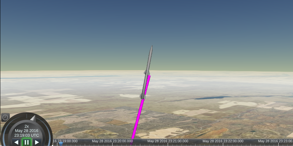
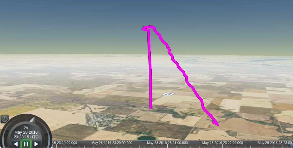
3D Flight Playback
After performing multiple test flights during development of Osprey, I was sitting on a large amount of orientation data (roll, pitch, and heading), but didn’t have any use for it. Certainly, it would be interesting to see the rocket’s orientation versus time graph of a flight. Additionally, given the GPS coordinates of the flight and the altitude, it would be interesting to see a 3D flight path rather than 2D one overlaid onto a flat map.
I was already working on an automatic flight report for quick post-flight analysis since reading through a JSON log file with a few thousand lines isn’t exactly user friendly. The Cesium project was exactly what I was looking for. I could put an instance in my HTML-based flight report, use the location and altitude data to plot a flight path in 3D and use a model of a rocket to replay the rocket’s orientation throughout the flight.
The code itself isn’t especially interesting unless you’re working with Cesium’s API so rather than go into detail about it here, I’ll just link to the relevant JS file on GitHub. What is interesting, however, is the final product. A sample flight report is available at https://shanet.github.io/Osprey. Below is a screenshot of the model of the rocket tilting slightly after liftoff which matches the actual behavior of that particular flight.
Future Additions & Conclusion
Given that my original vision for this project was a simple tracking system which then snowballed into much more than that and ended up taking eight months, I’m ready to switch gears to something else for a while. Nonetheless, I do have some future expansion ideas:
- “Micro version” with only a processor, IMU, and battery for data logging purposes only.
- The 3D flight path playback in the launch report could be made more rich with the addition of altitude and flight phase data.
- Support for multiple flight stages.
- Reworking the igniter circuit to only need a single capacitor.
- Support for offline maps in the generated launch report webpage.
Overall, it would have been orders of magnitude easier and cheaper to simply buy one of the many existing flight computers out there, but the amount of learning that resulted from this project is invaluable. I’ve never worked on something that included circuit design, embedded systems, mobile applications, desktop applications, web development, and everything in between. Of course, I’m sure that my future rockets will require additional features which means that I expect this project will grow alongside those rockets to support and fulfill their needs.
The full source and build instructions are available on GitHub.